ABSTRACT: By configuring the LFM, we are ready to solve the inverse problem.
In the previous page, we described the sensor array before introducing the lead field matrix (LFM).
The forward problem was solved by the Sarvas formula. Therefore, if the current moment and position of the current dipole are known, the magnetic field (sensor signal) at an arbitrary position can be obtained.
By the way, the output signal \( \boldsymbol{b} \) of the sensor array actually measured and the theoretical output signal \(\boldsymbol{\hat{b}} \) estimated by using the Sarvas formula differ due to various factors. In the discussion below, we will distinguish between the two.
From the discussion in the previous section, when we assume that the number of sensors is M and the estimated signal output of the mth sensor is \(\hat{b}_{m} \), the estimated signal output \( \boldsymbol{\hat{b}} \) from the sensor array using the Sarvas formula is represented as
$$ \boldsymbol{\hat{b}}=\left(\begin{array}{cccc}\hat{b}_{1} & \hat{b}_{2} & \ldots & \hat{b}_{M} \\\end{array}\right)^T $$
From the linearity between the current moment and magnetic field, the relationship of the two can be expressed as a matrix.
Therefore, we discuss the matrix \(\boldsymbol{L}\) when it is written as \(\boldsymbol{\hat{b}}=\boldsymbol{L}\boldsymbol{q}\).
The principle led from Sarvas formula shows that the sensor signal is linear to the current moment and is non-linear to the position. Such non-linearity requires us to explore the signal space.
Therefore, it is convinient to examine how the signal of each sensor react when the unit current moment at an arbitrary position. This reaction is generally called as an array response vector, but it is commonly called as a lead field in magnetoencephalography analysis [1]. The array response vector for each dimension is called as the lead field vector, which is integrated dimensionally to be called as the lead field matrix (LFM).
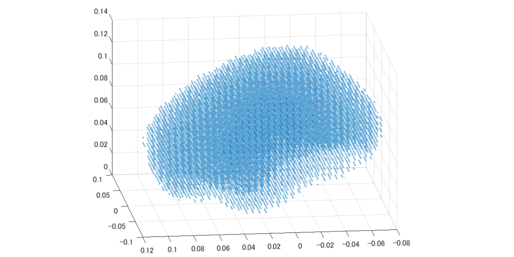
Now, we would like to consider dividing the brain into N grid points and measure magnetic fieled with M sensors. For example, when each grid point is created with 5 mm, the webmaster’s brain is divided into N = 14,000 grid points as the figure shown below.

Let \(\boldsymbol{L}_{n}\) be the LFM at the nth grid point when there are N grid points. Let us consider in Cartesian coordinates. We represent the column vector (array response vector) corresponding each dimension of xyz as \(\boldsymbol{l}_{n} ^x\), \(\boldsymbol{l}_{n} ^y\), and \(\boldsymbol{l}_{n} ^z\), respectively. Furthermore, we represent the scalar value of the magnetic field at the mth sensor for the unit current moment in the x-axis direction as \(l_{n_m}^x\), and the current moment of the current dipole at the nth grid point as \(\boldsymbol{q}_{n}\). It follows as
$$ \boldsymbol{L}_{n}=\left(\begin{array}{cccc}\boldsymbol{l}_{n}^x &\boldsymbol{l}_{n}^y &\boldsymbol{l}_{n}^z\\\end{array}\right)=\left(\begin{array}{cccc}l_{n_1}^x & l_{n_1}^y & l_{n_1}^z \\l_{n_2}^x & l_{n_2}^y & l_{n_2}^z \\\vdots & \vdots & \vdots \\l_{n_M}^x & l_{n_M}^y & l_{n_M}^z \\\end{array}\right) $$
$$ \boldsymbol{q}_{n}=\left(\begin{array}{cccc}q_{n}^x &q_{n}^y & q_{n}^z\\\end{array}\right)^T $$
The estimated output of each sensor can be obtained in a simple form as follows, which is the result of configuring LFM.
$$ \boldsymbol{\hat{b}}=\boldsymbol{L}_{n}\boldsymbol{q}_{n} $$
By the way, it seems that there is no problem solving the inverse problem by comparing the measured magnetic field \(\boldsymbol{b}\) and the estimated magnetic field \(\boldsymbol{\hat{b}}\). However, according to the Sarvas formula, the component of the current moment of the current dipole that is perpendicular to the center of the virtual sphere does not generate any magnetic field. In other words, even if the inverse problem is solved to estimate \(\boldsymbol{q}_{n}\), the vertical component cannot be discussed and must be removed.
Therefore, we should renew the forward problem from Cartesian coordinates to polar coordinates as follows
$$ \boldsymbol{L}_{n}=\left(\begin{array}{cccc}\boldsymbol{l}_{n}^\theta &\boldsymbol{l}_{n}^\phi & \boldsymbol{l}_{n}^r \\\end{array}\right) $$
$$ \boldsymbol{q}_{n}=\left(\begin{array}{cccc}q_{n}^\theta &q_{n}^\phi & q_{n}^r\\\end{array}\right)^T $$
However, \(\boldsymbol{l}_{n}^r\) is a zero vector and \(q_{n}^r\) cannot be discussed. After all, we can delete one dimension as follows
$$ \boldsymbol{L}_{n}=\left(\begin{array}{cccc}\boldsymbol{l}_{n}^\theta &\boldsymbol{l}_{n}^\phi \\\end{array}\right) $$
$$ \boldsymbol{q}_{n}=\left(\begin{array}{cccc}q_{n}^\theta &q_{n}^\phi \\\end{array}\right)^T $$
We continue the discussion about LFM in line with this idea.
It is also possible to select multiple grid points to form a LFM. For example, when selecting the a-th and b-th grid points, we can configure the LFM as
$$ \boldsymbol{L}_{ab}=\left(\begin{array}{cccc}\boldsymbol{l}_{a}^\theta &\boldsymbol{l}_{a}^\phi & \boldsymbol{l}_{b}^\theta&\boldsymbol{l}_{b}^\phi \\\end{array}\right) $$
$$ \boldsymbol{q}_{ab}=\left(\begin{array}{cccc}q_{a}^\theta &q_{a}^\phi & q_{b}^\theta &q_{b}^\phi \\\end{array}\right)^T $$
We can also estimate the magnetic field as
$$ \boldsymbol{\hat{b}}=\boldsymbol{L}_{ab}\boldsymbol{q}_{ab} $$
However, in Multi ECD estimation, it is difficult to calculate directly because we have to consider the combination to select the grid points. For example, the webmaster’s brain requires about 100 million ways to choose 2 from 14,000 grid points, and about 460 billion to choose 3 grid points. Techniques such as MUSIC algorithm are required.
It is also possible to configure a LFM with all grid points, which is the basic idea of a spatial filter. Since all grid points are selected, there is no need to think about combinations because there is only one combination to select all.
$$ \boldsymbol{L}_{all}=\left(\begin{array}{cccc}\boldsymbol{l}_{1}^\theta &\boldsymbol{l}_{1}^\phi & \ldots & \ldots & \boldsymbol{l}_{N}^\theta&\boldsymbol{l}_{N}^\phi \\\end{array}\right) $$
$$ \boldsymbol{q}_{all}=\left(\begin{array}{cccc}q_{1}^\theta & q_{1}^\phi & \ldots & \ldots & q_{N}^\theta & q_{N}^\phi \\\end{array}\right)^T $$
We can also estimate the magnetic field as
$$ \boldsymbol{\hat{b}}=\boldsymbol{L}_{all}\boldsymbol{q}_{all} $$
Now we are ready to solve the inverse problem.
SUMMARY: Now we are ready to solve the inverse problem by configuring the LFM.
In the next page, we will solve the inverse problem by comparing the measured magnetic field \(\boldsymbol{b}\) with the estimated magnetic field \( \boldsymbol{\hat{b}} \).
(Reference)
MS Hämäläinen, RJ Ilmoniemi: Interpreting magnetic fields of the brain: minimum norm estimates. Med Biol Eng Comput. 1994 Jan;32(1):35-42.