Abstract: The minimum norm estimate (MNE), a mathematical solution to the inverse problem of the underdetermined systems, did not fit the practice in the analysis, which motivated the development of the spatial filters.
In the previous page, we mentioned that the underdetermined solution is called variously.
Herein, we would like to start discussing the non-adaptive beamformers through the minimum norm estimate (MNE), a basical spatial filter. The solution is underdetermined and non-adaptive, so the target information is one sample (the signal output \(\boldsymbol{b}\) by the sensor array at a certain moment).
Assuming the linear mapping between the current moment \(\boldsymbol{q}\) and the magnetic field \(\boldsymbol{b}\) as the Lead Field Matrix (LFM) \( \boldsymbol{L} \) when the position of the current dipole is fixed. The following equation holds:
$$ \boldsymbol{b}=\boldsymbol{L}\boldsymbol{q} $$
Now we would like to find the inverse correspondence (inverse linear mapping) \(\boldsymbol{L}^{-}\) that estimates the current moment from the magnetic field.
$$ \boldsymbol{q}=\boldsymbol{L}^-\boldsymbol{b} $$
In principle, spatial filters assume that signals are generated from all parts of the signal space, so \(\boldsymbol{q}=\boldsymbol{q}_{all}\), \(\boldsymbol{L}=\boldsymbol{L}_{all}\).
The mathematical and underdetermined solution of
$$ \boldsymbol{b}=\boldsymbol{L}\boldsymbol{q} $$
is the following:
$$ \boldsymbol{q}=\boldsymbol{L}^{-}\boldsymbol{b}=\boldsymbol{L}^T(\boldsymbol{L}\boldsymbol{L}^{T})^{-1}\boldsymbol{b} $$
And the solution is called the Minimum Norm Estimate (MNE) due to the derivation process [1].
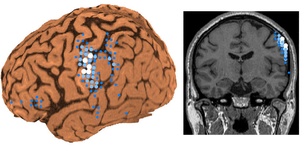
The MNE requires the overall signal as small as possible during the derivation process. Therefore, the obtained solution explains the sensor signal only by the lattice points close to the sensors. In other words, the current moment at the lattice points close to the sensors is relatively emphasized [2]. The analysis results in magnetoencephalography show signals scattered on the brain surface as shown in the figure below.

This is fine, but in actual MEG analysis, it is often necessary to assume the signal source as a single focus at a certain depth. In other words, MNE is often not suited to the practical situation of MEG analysis.
The reason why MNE does not fit the real brain activity is that the magnitude of the current moment depends on its position (the position of the lattice point to which the dipole belongs).
Let us rewrite the following MNE solution
$$ \boldsymbol{q}=\boldsymbol{L}^T(\boldsymbol{L}\boldsymbol{L}^{T})^{-1}\boldsymbol{b} $$
into
$$ \left(\begin{array}{cccc}\boldsymbol{q}_{1} \\ \vdots \\ \boldsymbol{q}_{N}\end{array}\right)=\left(\begin{array}{cccc}\boldsymbol{L}_{1}^{T} \\ \vdots \\ \boldsymbol{L}_{N}^{T}\end{array}\right) (\boldsymbol{L}\boldsymbol{L}^{T})^{-1}\boldsymbol{b} $$
Note the number of lattice points in the signal space (typically the whole brain) is N. Let us rewrite the followings as
$$ \boldsymbol{q}_{n}=\left(\begin{array}{cccc}q_{n}^{\theta} & q_{n}^{\phi} \end{array} \right)^{T} $$
$$ \boldsymbol{q}=\boldsymbol{q}_{all}=\left(\begin{array}{cccc}q_{1}^{\theta} & q_{1}^{\phi} & \ldots & \ldots & q_{N}^{\theta} & q_{N}^{\phi} \end{array} \right)^{T} $$
$$ \boldsymbol{L}_{n}=\left(\begin{array}{cccc}\boldsymbol{l}_{n}^{\theta} & \boldsymbol{l}_{n}^{\phi} \end{array} \right)= \left(\begin{array}{cccc} l_{n_1}^{\theta} & l_{n_1}^{\phi} \\ \vdots & \vdots \\ l_{n_M}^{\theta} & l_{n_M}^{\phi} \end{array} \right) $$
$$ \boldsymbol{L}=\boldsymbol{L}_{all}=\left(\begin{array}{cccc}\boldsymbol{L}_{1} & \ldots & \boldsymbol{L}_{N} \end{array} \right)= \left(\begin{array}{cccc}\boldsymbol{l}_{1}^{\theta} & \boldsymbol{l}_{1}^{\phi} & \ldots & \ldots & \boldsymbol{l}_{N}^{\theta} &\boldsymbol{l}_{N}^{\phi} \end{array} \right) $$
to get the following current moment in each lattice:
$$ \boldsymbol{q}_{n}=\boldsymbol{L}_{n}^T(\boldsymbol{L}\boldsymbol{L}^{T})^{-1}\boldsymbol{b} $$
Using the Frobenius norm, we obtain the following inequality due to the submultiplicative property of the norm:
$$ \|\boldsymbol{q}_{n}\|=\| \boldsymbol{L}_{n}^T(\boldsymbol{L}\boldsymbol{L}^{T})^{-1}\boldsymbol{b} \| \leq \| \boldsymbol{L}_{n}^T(\boldsymbol{L}\boldsymbol{L}^{T})^{-1}\|_{F} \| \boldsymbol{b} \| $$
Let us transform this into
$$ \frac{\|\boldsymbol{q}_{n}\|}{\|\boldsymbol{b} \|} \leq \| \boldsymbol{L}_{n}^T(\boldsymbol{L}\boldsymbol{L}^{T})^{-1}\|_{F} $$
Now we can see that the maximum magnitude of the current moment (relative to the magnitude of the measured magnetic field) depends on the LFM at each lattice point, which determines the distribution of the MNE solutions.
To escape from the curse of this maximum value, we need to create a new evaluation value, for example dividing the current moment by this magnitude to standardize it. This method is called Dynamic statistical parametric mapping (dSPM) or Weight (noise) normalized minimum norm filter [3].
Let us write the new generalized evaluation value for the n-th lattice point as \(\boldsymbol{q}_{n_{filtered}}\), and let the weighting matrix be \(\boldsymbol{W}_{n}^{T}\) corresponding to the linear inverse mapping \(\boldsymbol{L}_{n}^{-} \). Then,
$$ \boldsymbol{q}_{n_{MNE}}= \boldsymbol{q}_{n}=\boldsymbol{L}_{n}^T(\boldsymbol{L}\boldsymbol{L}^{T})^{-1}\boldsymbol{b} $$
$$ \boldsymbol{q}_{n_{filtered}}= \boldsymbol{W}_{n}^T\boldsymbol{b} $$
$$ \boldsymbol{W}_{n}=\left(\begin{array}{cccc} \boldsymbol{w}_{n}^{\theta} & \boldsymbol{w}_{n}^{\phi} \end{array} \right)= \left(\begin{array}{cccc} w_{n_1}^{\theta} & w_{n_1}^{\phi} \\ \vdots & \vdots \\ w_{n_M}^{\theta} & w_{n_M}^{\phi} \end{array} \right) $$
And we can rewrite them as follows:
$$ \boldsymbol{q}_{MNE}= \boldsymbol{q}=\boldsymbol{L}^T(\boldsymbol{L}\boldsymbol{L}^{T})^{-1}\boldsymbol{b} $$
$$ \boldsymbol{q}_{filtered}= \boldsymbol{W}^T\boldsymbol{b} $$
$$ \boldsymbol{W}^{T}= \left(\begin{array}{cccc} \boldsymbol{W}_{1}^{T} \\ \vdots \\ \boldsymbol{W}_{M}^{T} \end{array} \right) $$
Of course, the following holds for MNEs:
$$ \boldsymbol{W}^{T}=\boldsymbol{W}_{MNE}^{T}= \left(\begin{array}{cccc} \boldsymbol{L}_{1}^T(\boldsymbol{L}\boldsymbol{L}^{T})^{-1} \\ \vdots \\ \boldsymbol{L}_{N}^T(\boldsymbol{L}\boldsymbol{L}^{T})^{-1} \end{array} \right) =\boldsymbol{L}^T(\boldsymbol{L}\boldsymbol{L}^{T})^{-1} $$
By the way, solving the inverse problem should be to find the inverse linear mapping \( \boldsymbol{L}^{-} \) and determine the current moment \(\boldsymbol{q}\). In other words, it should be to find the following solution:
$$ \boldsymbol{q}=\boldsymbol{L}^{-}\boldsymbol{b} $$
However, the our objective shifted to constructing a spatial filter (calculating the weighting matrix \(\boldsymbol{W}^{T}\) and determining the evaluation value \(\boldsymbol{q}_{filtered}\)). In other words, our objective shifted to finding the following solution:
$$ \boldsymbol{q}_{filtered}= \boldsymbol{W}^T\boldsymbol{b} $$
It can be interpreted that the concept of solving an inverse problem has been extended to the construction of a spatial filter. It can also be interpreted that determining the current moment \(\boldsymbol{q}\) has been extended to determining the evaluation value \(\boldsymbol{q}_{filtered}\).
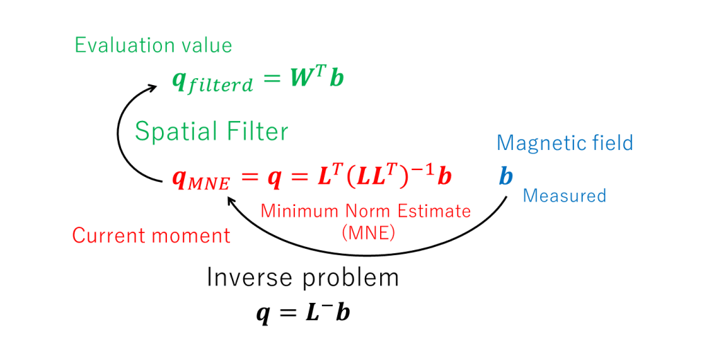
The evaluation value \(\boldsymbol{q}_{filtered}\) is a virtual value and can be flexibly proposed by devising the weighting matrix \(\boldsymbol{W}^{T}\). Constructing a spatial filter is nothing more than proposing a weighting matrix \(\boldsymbol{W}^{T}\) to propose an evaluation value \(\boldsymbol{q}_{filtered}\) that suits the purpose (see figure below).

Summary: The concept of solving the inverse problem in the underdetermined system has been extended to constructing the spatial filter.
In the next page, we would like to discuss representative non-adaptive beam formers: dSPM, sLORETA, and SMF.
(References)
- MS Hämäläinen, RJ Ilmoniemi: Interpreting magnetic fields of the brain: minimum norm estimates. Med Biol Eng Comput. 1994 Jan;32(1):35-42.
- Kensuke Sekihara, Maneesh Sahani, Srikantan S Nagarajan: Localization bias and spatial resolution of adaptive and non-adaptive spatial filters for MEG source reconstruction. Neuroimage. 2005 May 1;25(4):1056-67.
- AM Dale, AK Liu, BR Fischl, RL Buckner, JW Belliveau, JD Lewine, E Halgren: Dynamic statistical parametric mapping: combining fMRI and MEG for high-resolution imaging of cortical activity. Neuron. 2000 Apr;26(1):55-67.