Abstract: The Adaptive Beamformer handles time width to exceed the limitations of the Non-adaptive Beamformer that handles time sample.
We started by finding the inverse linear mapping \( \boldsymbol{L}^{-} \) and determining the current moment \( \boldsymbol{q}\) to solve the inverse problem of the underdetermined system.
$$ \boldsymbol{q}=\boldsymbol{L}^-\boldsymbol{b} $$
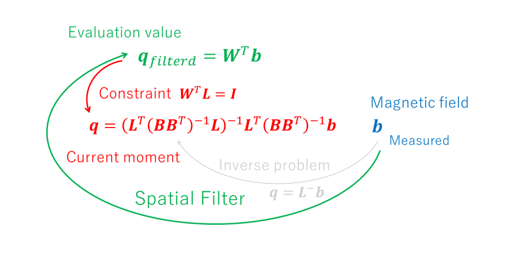
However, we found that this mathematical solution (Minimum Norm Estimate (MNE)) did not fit the practice of magnetoencephalography analysis. To overcome this situation, we extended the concept of solving the inverse problem to constructing a spatial filter. In this way, we obtained the weighting matrix \(\boldsymbol{W}^{T}\) and determined the evaluation value \(\boldsymbol{q}_{filtered}\).
$$ \boldsymbol{q}_{filtered}= \boldsymbol{W}^T\boldsymbol{b} $$
By the way, the following holds in the forward solution:
$$ \boldsymbol{b}=\boldsymbol{Lq} $$
A spatial filter can also be expressed as
$$ \boldsymbol{q}_{filtered}= \boldsymbol{W}^T\boldsymbol{Lq} $$
If
$$ \boldsymbol{W}^T\boldsymbol{L}=\boldsymbol{I} $$
the meaning of the evaluation value \(\boldsymbol{q}_{filtered}\) goes back to the current moment \(\boldsymbol{q}\).
$$ \boldsymbol{q}_{filtered}= \boldsymbol{q} $$
We would like to consider constructing a better spatial filter under this constraint \(\boldsymbol{W}^T\boldsymbol{L}=\boldsymbol{I}\) (see figure below).

In the previous page, various proposals were made for non-adaptive beamformers, such as MNE, dSPM, sLORETA, and SMF, but in the end, they could not escape the curse of underdetermined solutions, and each has its own advantages and disadvantages, which made the discussion seem limited.
An underdetermined solution is a state of information underload, and the natural solution is to add more information to overcome this situation. Considering that the information handled by the non-adaptive beamformer is only a moment in time (one sample on the time axis), it is possible to handle a certain time span (a series of multiple samples on the time axis).
From now on, instead of just one time sample, we will consider the time span \(t=t_1,t_2, \ldots, t_K\) as follows:
$$ \boldsymbol{B}=\left(\begin{array}{cccc} \boldsymbol{b}_{t=t_1} & \boldsymbol{b}_{t=t_2} & \ldots & \boldsymbol{b}_{t=t_K} \end{array} \right) $$
$$ \boldsymbol{q}_{n}^{\theta}=\left(\begin{array}{cccc} q_{n_{t=t_1}}^{\theta} & q_{n_{t=t_2}}^{\theta} & \ldots & q_{n_{t=t_K}}^{\theta} \end{array} \right) $$
$$ \boldsymbol{q}_{n}^{\phi}=\left(\begin{array}{cccc} q_{n_{t=t_1}}^{\phi} & q_{n_{t=t_2}}^{\phi} & \ldots & q_{n_{t=t_K}}^{\phi} \end{array} \right) $$
$$ \boldsymbol{Q}_{n}=\left(\begin{array}{cccc}\boldsymbol{q}_{n}^{\theta} \\ \boldsymbol{q}_{n}^{\phi} \end{array} \right) $$
Previously we considered the magnetic field about one time sample under the constraint \(\boldsymbol{b}=\boldsymbol{Lq}\) to minimize to the magnitude of the current moment \( \|\boldsymbol{q}\|^2 \).
$$ \boldsymbol{q}=\underset{\boldsymbol{q}}{\arg\min}\|\boldsymbol{q}\|^2 \hspace{10pt} subject \hspace{5pt}to\hspace{10pt}\boldsymbol{b}=\boldsymbol{Lq} $$
Now it is natural extension for us to consider the magnetic field about time span under the constraint \(\boldsymbol{W}^T\boldsymbol{L}=\boldsymbol{I}\) to minimize to the power of the sequential current moment \( \|\boldsymbol{Q}\|^2 \).
That is, consider the power in the \(\theta\) direction of the n-th lattice point, \(\frac{1}{K}\|\boldsymbol{q}_{n}^{\theta}\|^2\) (the \(\phi\) direction is similar and will be omitted).
Considering this minimization is equivalent to considering minimization of \(\|\boldsymbol{q}_{n}^{\theta}\|^2=\|\boldsymbol{w}_{n}^{\theta^{T}}\boldsymbol{B}\|^2\), with \(\frac{1}{K}\) omitted. So we would like to consider the later.
This technique is called Minimum Variance Spatial Filter, Minimum Variance Beamformer (MVBF), or Linearly Constrained Minimum Variance Beamformer [1].
Note that if we do not omit \(\frac{1}{K}\), \(\frac{1}{K}\boldsymbol{BB}^{T}\) is the covariance matrix of \(\boldsymbol{B}\). Therefore, in some articles, \(\boldsymbol{BB}^{T}\) in the equation below is written as \(Cov(\boldsymbol{B})\), \(\boldsymbol{\Sigma}\), or \(\boldsymbol{R}\).
For lattice point n, if we handle \(\theta\) and \(\phi\) together, we need to consider minimizing \(\|\boldsymbol{Q}_{n}\|_{F}^2=\|\boldsymbol{W}_{n}^{T}\boldsymbol{B}\|_{F}^2\).
Note that regarding the constraints, only the information \(\boldsymbol{W}_{n}^{T}\boldsymbol{L}_{n}=\boldsymbol{I}_{2}\) out of \(\boldsymbol{W}^T\boldsymbol{L}=\boldsymbol{I}\) is used (a necessary condition). In other words, conditions other than the diagonal elements and those before and after them are not used. Therefore, it is necessary to evaluate whether the constraints are satisfied (whether \(\boldsymbol{W}^T\boldsymbol{L}\) is close to a unit matrix).
$$ \boldsymbol{W}_{n}^{T}=\underset{\boldsymbol{W}_{n}^{T}}{\arg\min}\|\boldsymbol{W}_{n}^{T}\boldsymbol{B}\|_{F}^2 \hspace{10pt} subject \hspace{5pt}to\hspace{10pt}\boldsymbol{W}_{n}^{T}\boldsymbol{L}_{n}=\boldsymbol{I}_{2} $$
As in the MNE solution, we use the Lagrange multiplier method. Namely, we introduce the Lagrange multiplier of \(\boldsymbol{\Lambda}\) and the Lagrange function of \(F(\boldsymbol{W}_{n}^{T},\boldsymbol{\Lambda})\), then
$$ F(\boldsymbol{W}_{n}^{T},\boldsymbol{\Lambda})=tr(\boldsymbol{W}_{n}^{T}\boldsymbol{BB}^{T}\boldsymbol{W}_{n}-(\boldsymbol{W}_{n}^{T}\boldsymbol{L}_{n}-\boldsymbol{I}_{2})\boldsymbol{\Lambda}) $$
When \(\|\boldsymbol{Q}_{n}\|_{F}^2=\|\boldsymbol{W}_{n}^{T}\boldsymbol{B}\|_{F}^2\) takes the minimum value,
$$ \frac{\partial F(\boldsymbol{W}_{n}^{T},\boldsymbol{\Lambda})}{\partial \boldsymbol{W}_{n}^{T}}=2\boldsymbol{W}_{n}^{T}\boldsymbol{BB}^{T}-\boldsymbol{\Lambda}^{T}\boldsymbol{L}_{n}^{T}=\boldsymbol{O} $$
$$ \frac{\partial F(\boldsymbol{W}_{n}^{T},\boldsymbol{\Lambda})}{\partial \boldsymbol{\Lambda}}=(\boldsymbol{W}_{n}^{T}\boldsymbol{L}_{n}-\boldsymbol{I}_{2})^{T}=\boldsymbol{O} $$
Therefore,
$$ \boldsymbol{W}_{n}^{T}=\frac{\boldsymbol{\Lambda}^{T}}{2}\boldsymbol{L}_{n}^{T}(\boldsymbol{BB}^{T})^{-1} $$
Hence,
$$ \boldsymbol{W}_{n}^{T}\boldsymbol{L}_{n}=\frac{\boldsymbol{\Lambda}^{T}}{2}\boldsymbol{L}_{n}^{T}(\boldsymbol{BB}^{T})^{-1}\boldsymbol{L}_{n}=\boldsymbol{I}_{2} $$
So it is solved as
$$ \boldsymbol{\Lambda}^{T}=2(\boldsymbol{L}_{n}^{T}(\boldsymbol{BB}^{T})^{-1}\boldsymbol{L}_{n})^{-1} $$
$$ \boldsymbol{W}_{n}^{T}=(\boldsymbol{L}_{n}^{T}(\boldsymbol{BB}^{T})^{-1}\boldsymbol{L}_{n})^{-1}\boldsymbol{L}_{n}^{T}(\boldsymbol{BB}^{T})^{-1} $$
Furthermore, we can also solve the following situation:
$$ \boldsymbol{W}^{T}=\underset{\boldsymbol{W}^{T}}{\arg\min}\|\boldsymbol{W}^{T}\boldsymbol{B}\|_{F}^2 \hspace{10pt} subject \hspace{5pt}to\hspace{10pt}\boldsymbol{W}^{T}\boldsymbol{L}=\boldsymbol{I} $$
if we use \( \boldsymbol{W}_{n}^{T}\to\boldsymbol{W}^{T} \), \(\boldsymbol{L}_{n}\to\boldsymbol{L}\), and \(\boldsymbol{I}_{2}\to\boldsymbol{I}\), we can solve \( \boldsymbol{W}^{T}\) directly as follows:
$$ \boldsymbol{\Lambda}^{T}=2(\boldsymbol{L}^{T}(\boldsymbol{BB}^{T})^{-1}\boldsymbol{L})^{-1} $$
$$ \boldsymbol{W}^{T}=(\boldsymbol{L}^{T}(\boldsymbol{BB}^{T})^{-1}\boldsymbol{L})^{-1}\boldsymbol{L}^{T}(\boldsymbol{BB}^{T})^{-1} $$
Actually, this expression is used in van Veen article [1].
However, when it is put into practice, \((\boldsymbol{L}^{T}(\boldsymbol{BB}^{T})^{-1}\boldsymbol{L})^{-1}\) is a difficult task because it requires finding the inverse matrix from \(\boldsymbol{L}^{T}(\boldsymbol{BB}^{T})^{-1}\boldsymbol{L}\), which is 2Nx2N matrix (28,000×28,000 in the webmaster’s brain).
If we calculate the elements \(\boldsymbol{W}_{n}^{T}\) of the weight matrix \(\boldsymbol{W}^{T}\) to avoid the problem above, we only use a part of the constraint \(\boldsymbol{W}^T\boldsymbol{L}=\boldsymbol{I}\) as a necessary condition. In the calculation, only the diagonal elements and the elements before and after them of the 2Nx2N unit matrix are used as conditions.
If each weight vector and any lead field vector are always independent, then all the rest of the constraint \(\boldsymbol{W}^T\boldsymbol{L}=\boldsymbol{I}\) is zero. (Any lead vector other than (\boldsymbol{l}_{n}^{\theta}\) is denoted as \(\boldsymbol{l}_{k}^{\omega}\).)
$$ \boldsymbol{w}_{n}^{\theta^{T}}\boldsymbol{l}_{k}^{\omega}=0 $$
However, it is strongly expected that this will not be realized, because it is not realistic to always have all 2N-1=28,000-1 lead vectors independent for each of the 2N=28,000 weight vectors. Therefore, it is necessary to evaluate the values other than the diagonal elements of \(\boldsymbol{W}^T\boldsymbol{L}=\boldsymbol{I}\).
On the other hand, if we directly calculate \( \boldsymbol{W}^{T}\), some computational ingenuity is required to calculate the inverse matrix \((\boldsymbol{L}^{T}(\boldsymbol{BB}^{T})^{-1}\boldsymbol{L})^{-1}\) (since it is not realistic to expect all 2N=28,000 vectors to be independent).
Since these are ultimately dealing with the same problem, it is not true that one method is better than the other. However, in order to save on computational effort, it seems common to calculate \(\boldsymbol{W}_{n}^{T}\) and evaluate the non-diagonal elements of \(\boldsymbol{W}^T\boldsymbol{L}=\boldsymbol{I}\).
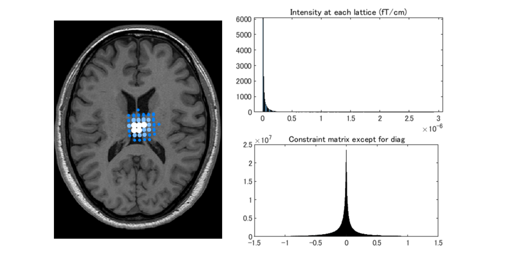
By the way, if we construct \(\boldsymbol{W}^{T}\) and apply it to the analysis (without thinking about it), we will get the figure below.

As shown in the upper right figure, the distribution (histogram) of signal intensity (magnitude of current moment) was steeply skewed to the right (the top five were 2,922 nAm, 1,725 nAm, 1,521 nAm, 1,286 nAm, and 1,225 nAm, respectively). As shown in the lower right figure, the histogram for each component of \(\boldsymbol{W}^T\boldsymbol{L}-\boldsymbol{I}\), obtained by subtracting the right side from the left side of the constraint, showed that the constraint \(\boldsymbol{W}^T\boldsymbol{L}\) was close to an identity matrix. However, the analysis results point to the center of the brain. No matter which sample we tried to choose, simply applying MVBF only resulted in an image where the center of the brain was bright.
Due to the characteristics of the Sarvas formula, which is the basis of magnetoencephalography analysis, the current dipole does not generate any magnetic field at the center of the virtual sphere. In other words, since all components of the lead field \(\boldsymbol{L}_{n}\) are zero at the center of the brain, all components of the weight \(\boldsymbol{W}_{n}^{T}\) that satisfies the constraint \(\boldsymbol{W}_{n}^T\boldsymbol{L}_{n}=\boldsymbol{I}\) diverge to infinity.
In such situation, the current moment also diverges to infinity, as shown below. In other words, analysis is not possible near the center of the brain.
$$ \boldsymbol{q}_{n}=\boldsymbol{W}_{n}^{T}\boldsymbol{b} $$
This result is in contrast to the non-adaptive beamformer MNE, which always produced images in which the brain surface was illuminated. Simple MVBF just produces illuminated center regardless of the sample which was useless and worse than MNE.
As we reviewed above, MVBF is a good idea, but due to the characteristics of the Sarvas formula, which is the basis of magnetoencephalography analysis, it will always fail if applied simply.
Summary: MVBF, an adaptive beamformer, is useless when simply applied to magnetoencephalography analysis.
In the next page, we would like to consider ways to adapt MVBF to practical analyses.
(References)
- BD van Veen, W van Drongelen, M Yuchtman, A Suzuki: Localization of brain electrical activity via linearly constrained minimum variance spatial filtering. IEEE Trans Biomed Eng. 1997 Sep;44(9):867-80.