Abstract: The Adaptive beamformer in magnetoencephalography is a modification of the minimum variance beamformer (MVBF). The methods includes modified signal space constructed using a brain surface mesh or a brain with the center hollowed out. Other proposed methods include array-grain / weight normalized minimum variance filter and synthetic aperture magnetometry (SAM), etc.
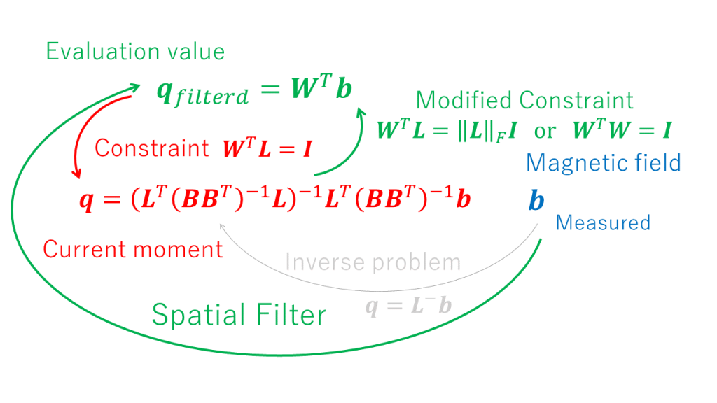
In the previous page, we attempted to obtain a Minimum variance beamformer (MVBF) to propose a weighting matrix that goes beyond the limitations of a non-adaptive beamformer by inputting time span information about the measured magnetic field.
That is, we solved
$$ \boldsymbol{W}_{n}^{T}=\underset{\boldsymbol{W}_{n}^{T}}{\arg\min}\|\boldsymbol{W}_{n}^{T}\boldsymbol{B}\|_{F}^2 \hspace{10pt} subject \hspace{5pt}to\hspace{10pt}\boldsymbol{W}_{n}^{T}\boldsymbol{L}_{n}=\boldsymbol{I}_{2} $$
and obtained the following [1]
$$ \boldsymbol{W}_{n}^{T}=(\boldsymbol{L}_{n}^{T}(\boldsymbol{BB}^{T})^{-1}\boldsymbol{L}_{n})^{-1}\boldsymbol{L}_{n}^{T}(\boldsymbol{BB}^{T})^{-1} $$
However, due to the characteristics of the Sarvas formula, the signal strength at the center (and its vicinity) of the virtual sphere was always huge, so the result was not useful as a spatial filter.
A simple solution to this situation is to construct a signal space that avoids the center of the virtual sphere. Next, we can modify the constraints to standardize the components of \(\boldsymbol{L}_{n}\) so that they do not all become zero at the center of the virtual sphere, or conversely, to standardize the components of \(\boldsymbol{W}_{n}^{T}\) so that they do not diverge to infinity.

That is,
- To remove the area near the center of the virtual sphere (hollow out the center of the brain) in the signal space (the space whrere the lattice points constructing the LFM are assumed; in magnetoencephalography, this is usually the brain itself).
- To modify the constraint \(\boldsymbol{W}_{n}^{T}\boldsymbol{L}_{n}=\boldsymbol{I}_{2}\) to \(\boldsymbol{W}_{n}^{T}\boldsymbol{L}_{n}=\|\boldsymbol{L}_{n}\|_{F}\boldsymbol{I}_{2}\).
- To modify the constraint \(\boldsymbol{W}_{n}^{T}\boldsymbol{L}_{n}=\boldsymbol{I}_{2}\) to \(\boldsymbol{W}_{n}^{T}\boldsymbol{W}_{n}=\boldsymbol{I}_{2}\).
Solution 1 is a simple method, and if the center is hollowed out appropriately, there will be no problem. However, how much to hollow out is subjective. If it is hollowed out too much, the area where the signal source should exist will be hollowed out. If it is hollowed out too little, the solution will still be estimated in the center.
As an ultimate method of hollowing out, it is possible to construct the signal space only from the brain surface mesh. (I do not like this method and have no experience with it. I think we do not need additional surfice analysis any more because we use gradient magnetic-field topography (GMFT) that assums signal space only in the brain surface mesh [2].) This method may not be a problem if you use an analysis method that extracts only the cortex of the brain surface by image processing and constructs the LFM.
Solution 2 is a method to prevent all components of \(\boldsymbol{L}_{n}\) from becoming zero, and is called the array-gain minimum variance filter [3]. In other words, introducing \(\boldsymbol{\tilde{L}}_{n}=\frac{\boldsymbol{L}_{n}}{\|\boldsymbol{L}_{n}\|_{F}}\), we solve the following in the same way as MVBF:
$$ \boldsymbol{W}_{n}^{T}=\underset{\boldsymbol{W}_{n}^{T}}{\arg\min}\|\boldsymbol{W}_{n}^{T}\boldsymbol{B}\|_{F}^2 \hspace{10pt} subject \hspace{5pt}to\hspace{10pt}\boldsymbol{W}_{n}^{T}\boldsymbol{\tilde{L}}_{n}=\boldsymbol{I}_{2} $$
to obtain the followings
$$ \boldsymbol{W}_{n}^{T}=(\boldsymbol{\tilde{L}}_{n}^{T}(\boldsymbol{BB}^{T})^{-1}\boldsymbol{\tilde{L}}_{n})^{-1}\boldsymbol{\tilde{L}}_{n}^{T}(\boldsymbol{BB}^{T})^{-1} $$
$$ \boldsymbol{\tilde{L}}_{n}=\frac{\boldsymbol{L}_{n}}{\|\boldsymbol{L}_{n}\|_{F}} $$
The units of the evaluation value \(\boldsymbol{q}_{filtered}\) are fT or fT/cm.
As discussed in MVBF, we can directly compute \(\boldsymbol{W}^{T}\). In practice, we will compute \(\boldsymbol{W}_{n}^{T}\) and evaluate the constraint \(\boldsymbol{W}^{T}\boldsymbol{\tilde{L}}=\boldsymbol{I}\).
Solution 3 is a method to prevent the components of \(\boldsymbol{W}_{n}^{T}\) from diverging to infinity, and is called the Weight normalized minimum-variance filter, Unit noise-gain minimum-variance filter, Noise-normalized filter, Borgiotti-Kaplan beamformer, etc. [3].
In this case, the optimization is to solve
$$ \boldsymbol{\tilde{W}}_{n}^{T}=\underset{\boldsymbol{\tilde{W}}_{n}^{T}}{\arg\min}\|\boldsymbol{\tilde{W}}_{n}^{T}\boldsymbol{B}\|_{F}^2 \hspace{10pt} subject \hspace{5pt}to\hspace{10pt}\boldsymbol{\tilde{W}}_{n}^{T}\boldsymbol{\tilde{W}}_{n}=\boldsymbol{I}_{2} $$
Let \(\xi_{\theta}(>0),\xi_{\phi}(>0)\) obtained from \(\boldsymbol{\tilde{W}}_{n}^{T}\boldsymbol{\tilde{W}}_{n}=\boldsymbol{I}_{2}\) be as follows:
$$ \boldsymbol{\tilde{W}}_{n}^{T}\boldsymbol{L}_{n}=\left(\begin{array}{cccc} \xi_{\theta} & 0 \\ 0 & \xi_{\phi} \end{array} \right)=\boldsymbol{\Xi}_{2} $$
The optimization can be expressed as
$$ \boldsymbol{\tilde{W}}_{n}^{T}=\underset{\boldsymbol{\tilde{W}}_{n}^{T}}{\arg\min}\|\boldsymbol{\tilde{W}}_{n}^{T}\boldsymbol{B}\|_{F}^2 \hspace{10pt} subject \hspace{5pt}to\hspace{10pt}\boldsymbol{\tilde{W}}_{n}^{T}\boldsymbol{L}_{n}=\boldsymbol{\Xi}_{2} $$
As in the MVBF solution, assuming the Lagrange multiplier is \(\boldsymbol{\Lambda}\) and the Lagrange function is \(F(\boldsymbol{\tilde{W}}_{n}^{T},\boldsymbol{\Lambda})\), then
$$ F(\boldsymbol{\tilde{W}}_{n}^{T},\boldsymbol{\Lambda})=tr(\boldsymbol{\tilde{W}}_{n}^{T}\boldsymbol{BB}^{T}\boldsymbol{\tilde{W}}_{n}-(\boldsymbol{\tilde{W}}_{n}^{T}\boldsymbol{L}_{n}-\boldsymbol{\Xi}_{2})\boldsymbol{\Lambda}) $$
When \(\|\boldsymbol{Q}_{n}\|_{F}^2=\|\boldsymbol{\tilde{W}}_{n}^{T}\boldsymbol{B}\|_{F}^2\) takes a minimum value,
$$ \frac{\partial F(\boldsymbol{\tilde{W}}_{n}^{T},\boldsymbol{\Lambda})}{\partial \boldsymbol{\tilde{W}}_{n}^{T}}=2\boldsymbol{\tilde{W}}_{n}^{T}\boldsymbol{BB}^{T}-\boldsymbol{\Lambda}^{T}\boldsymbol{L}_{n}^{T}=\boldsymbol{O} $$
$$ \frac{\partial F(\boldsymbol{\tilde{W}}_{n}^{T},\boldsymbol{\Lambda})}{\partial \boldsymbol{\Lambda}}=(\boldsymbol{\tilde{W}}_{n}^{T}\boldsymbol{L}_{n}-\boldsymbol{\Xi}_{2})^{T}=\boldsymbol{O} $$
So,
$$ \boldsymbol{\tilde{W}}_{n}^{T}=\frac{\boldsymbol{\Lambda}^{T}}{2}\boldsymbol{L}_{n}^{T}(\boldsymbol{BB}^{T})^{-1} $$
Therefore,
$$ \boldsymbol{\tilde{W}}_{n}^{T}\boldsymbol{L}_{n}=\frac{\boldsymbol{\Lambda}^{T}}{2}\boldsymbol{L}_{n}^{T}(\boldsymbol{BB}^{T})^{-1}\boldsymbol{L}_{n}=\boldsymbol{\Xi}_{2} $$
Hence,
$$ \boldsymbol{\Lambda}^{T}=2\boldsymbol{\Xi}_{2}(\boldsymbol{L}_{n}^{T}(\boldsymbol{BB}^{T})^{-1}\boldsymbol{L}_{n})^{-1} $$
$$ \boldsymbol{\tilde{W}}_{n}^{T}=\boldsymbol{\Xi}_{2}(\boldsymbol{L}_{n}^{T}(\boldsymbol{BB}^{T})^{-1}\boldsymbol{L}_{n})^{-1}\boldsymbol{L}_{n}^{T}(\boldsymbol{BB}^{T})^{-1} $$
To simplify above, we introduce
$$ \boldsymbol{\Omega}=(\boldsymbol{L}_{n}^{T}(\boldsymbol{BB}^{T})^{-1}\boldsymbol{L}_{n})^{-1}\boldsymbol{L}_{n}^{T}(\boldsymbol{BB}^{T})^{-2}\boldsymbol{L}_{n}(\boldsymbol{L}_{n}^{T}(\boldsymbol{BB}^{T})^{-1}\boldsymbol{L}_{n})^{-1} $$
According to the relationship
$$ \boldsymbol{\tilde{W}}_{n}^{T}\boldsymbol{\tilde{W}}_{n}=\boldsymbol{I}_{2} $$
It holds
$$ \boldsymbol{\tilde{W}}_{n}^{T}\boldsymbol{\tilde{W}}_{n}=\boldsymbol{\Xi}_{2}\boldsymbol{\Omega}\boldsymbol{\Xi}_{2}^{T}=\boldsymbol{I}_{2} $$
And it also holds
$$ \boldsymbol{\Xi}_{2}=\boldsymbol{\Xi}_{2}^{T}=\left(\begin{array}{cccc} \xi_{\theta} & 0 \\ 0 & \xi_{\phi} \end{array} \right), \boldsymbol{\Xi}_{2}^{-1}=\boldsymbol{\Xi}_{2}^{T^{-1}}=\left(\begin{array}{cccc} \frac{1}{\xi_{\theta}} & 0 \\ 0 & \frac{1}{\xi_{\phi}} \end{array} \right) $$
Therefore, we can obtain \(\xi_{\theta}(>0),\xi_{\phi}(>0)\) as follows:
$$ \boldsymbol{\Xi}_{2}^{2}=\left(\begin{array}{cccc} \xi_{\theta}^{2} & 0 \\ 0 & \xi_{\phi}^{2} \end{array} \right)=\boldsymbol{\Omega}^{-1} $$
To extract diagonal components, we introduce
$$ \boldsymbol{f}_{\theta}^{T}=\left(\begin{array}{cccc} 1 & 0 \end{array} \right), \boldsymbol{f}_{\phi}^{T}=\left(\begin{array}{cccc} 0 & 1 \end{array} \right) $$
Then, it can be solved as follows:
$$ \boldsymbol{\Omega}=(\boldsymbol{L}_{n}^{T}(\boldsymbol{BB}^{T})^{-1}\boldsymbol{L}_{n})^{-1}\boldsymbol{L}_{n}^{T}(\boldsymbol{BB}^{T})^{-2}\boldsymbol{L}_{n}(\boldsymbol{L}_{n}^{T}(\boldsymbol{BB}^{T})^{-1}\boldsymbol{L}_{n})^{-1} $$
$$ \xi_{\theta}=\sqrt{\boldsymbol{f}_{\theta}^{T}\boldsymbol{\Omega}^{-1}\boldsymbol{f}_{\theta}} $$
$$ \xi_{\phi}=\sqrt{\boldsymbol{f}_{\phi}^{T}\boldsymbol{\Omega}^{-1}\boldsymbol{f}_{\phi}} $$
$$ \boldsymbol{\tilde{W}}_{n}^{T}=\left(\begin{array}{cccc} \boldsymbol{\tilde{w}}_{n}^{\theta^{T}} \\ \boldsymbol{\tilde{w}}_{n}^{\phi^{T}} \end{array} \right)=\left(\begin{array}{cccc} \xi_{\theta} & 0 \\ 0 & \xi_{\phi} \end{array} \right)(\boldsymbol{L}_{n}^{T}(\boldsymbol{BB}^{T})^{-1}\boldsymbol{L}_{n})^{-1}\boldsymbol{L}_{n}^{T}(\boldsymbol{BB}^{T})^{-1} $$
The units of the evaluation value \(\boldsymbol{q}_{filtered}\) are fT or fT/cm.
As in the discussion of MVBF, when directly solving for \(\boldsymbol{\tilde{W}}^{T}\), the solution is \(\boldsymbol{\tilde{W}}_{n}^{T}\to\boldsymbol{\tilde{W}}^{T}\), \(\boldsymbol{L}_{n}\to\boldsymbol{L}\), \(\boldsymbol{\Xi}_{2}\to\boldsymbol{\Xi}\), \(\boldsymbol{f}_{\theta},\boldsymbol{f}_{\phi}\to\boldsymbol{f}_{1},\boldsymbol{f}_{2},\ldots,\boldsymbol{f}_{2N}\)
In practice, we will solve \(\boldsymbol{\tilde{W}}_{n}^{T}\) and evaluate the constraint \(\boldsymbol{\tilde{W}}^{T}\boldsymbol{\tilde{W}}=\boldsymbol{I}\).
There are many other adaptive beamformers available, such as Synthetic Aperture Magnetometry (SAM), which takes background activity into account [4].
Summary: The Adaptive Beamformer is an excellent spatial filter, but it is advisable to use it with caution validating the quality of the information you put into it.
(References)
- BD van Veen, W van Drongelen, M Yuchtman, A Suzuki: Localization of brain electrical activity via linearly constrained minimum variance spatial filtering. IEEE Trans Biomed Eng. 1997 Sep;44(9):867-80.
- A Hashizume, K Iida, H Shirozu, R Hanaya, Y Kiura, K Kurisu, H Otsubo: Gradient magnetic-field topography for dynamic changes of epileptic discharges. Brain Res. 2007 May 4;1144:175-9.
- K Sekihara, SS Nagarajan, D Poeppel, A Marantz, Y Miyashita: Reconstructing spatio-temporal activities of neural sources using an MEG vector beamformer technique. IEEE Trans Biomed Eng. 2001 Jul;48(7):760-71.
- M Taniguchi, A Kato, N Fujita, M Hirata, H Tanaka, T Kihara, H Ninomiya, N Hirabuki, H Nakamura, S E Robinson, D Cheyne, T Yoshimine: Movement-related desynchronization of the cerebral cortex studied with spatially filtered magnetoencephalography. Neuroimage. 2000 Sep;12(3):298-306.