Abstract: The number of lattice points considered in the spatial filter covers all the space in which signals can exist (typically the entire brain) and is overwhelmingly greater than the number of sensors. Therefore, the inverse solution can be obtained formulaically and analytically in the underdetermined system.
In the previous page, we sought an overdetermined solution that can be applied when there are only a small number of current dipoles, such as when a part of the brain is assumed to have strong activity that dominates whole brain activity.
Next, we would like to find an underdetermined solution that can be applied when there are a large number of current dipoles, such as when the entire brain is assumed to be active.
Assuming the positions of the current dipoles are fixed, and that the LFM is \( \boldsymbol{L} \), the linear mapping between the current moment \(\boldsymbol{q}\) and the magnetic field \(\boldsymbol{b}\) is as follows:
$$ \boldsymbol{b}=\boldsymbol{L}\boldsymbol{q} $$
We would like to find the inverse correspondence (inverse linear mapping) \(\boldsymbol{L}^{-}\) to estimate the current moment from the magnetic field.
$$ \boldsymbol{q}=\boldsymbol{L}^-\boldsymbol{b} $$
Assuming the number of sensor arrays is M and the number of lattice points is N, and the number of points constituting the LFM is \(N_{LFM}\), then \(\boldsymbol{b}\) is an M-dimensional column vector, \(\boldsymbol{q}\) is a \(2N_{LFM}\)-dimensional column vector, and \( \boldsymbol{L} \) is a matrix of \( M\times2L_{LFM} \).
So far, this is the same as the previous page.
In principle, spatial filters assume that there is a current dipole at each of the many lattice points throughout the brain, generating a magnetic field. The situation where \(M<2N_{LFM}\) (M=204 or 306, whereas N>10,000 for a 5mm voxel of the whole brain) is called an underdetermined system, which is a state of information underload.
This system might be similar to the physiological activity of the brain than single-dipole estimation, which assumes a single current dipole. However, the disadvantage is that the spatial resolution is low due to the underdetermined system. Nevertheless, spatial filters are often used in fundamental research due to its flexibility.
In the following, we will consider estimating the current moment \( \boldsymbol{q} \) for all N lattice points. Then, \(N_{LFM}=N\), and
$$ \boldsymbol{L}=\boldsymbol{L}_{all}=\left(\begin{array}{cccc}\boldsymbol{l}_{1}^\theta&\boldsymbol{l}_{1}^\phi & \ldots & \ldots & \boldsymbol{l}_{N}^\theta &\boldsymbol{l}_{N}^\phi \\\end{array}\right) $$
$$ \boldsymbol{q}=\boldsymbol{q}_{all}=\left(\begin{array}{cccc}q_{1}^\theta & q_{1}^\phi & \ldots & \ldots & q_{N}^\theta & q_{N}^\phi \\\end{array}\right)^T $$
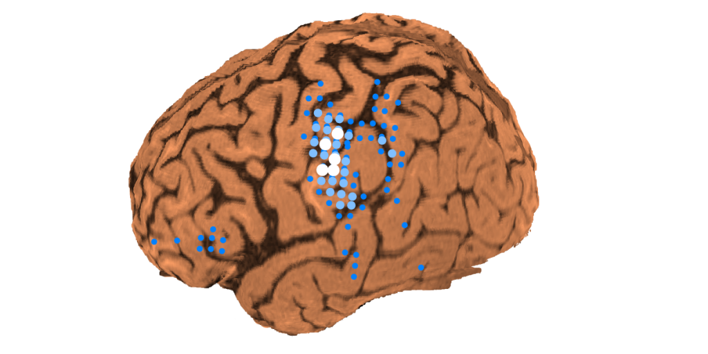
If we estimate the current moment of all lattice points \(\boldsymbol{q}=\boldsymbol{q}_{all} \) from the measured magnetic field \(\boldsymbol{b} \), we can draw a diagram like the one below. For the top 1% of current moments, the grid points with larger current moments are displayed larger and whiter.

In an underdetermined system, the measured magnetic field \( \boldsymbol{b} \) and the estimated magnetic field \( \boldsymbol{\hat{b}}=\boldsymbol{Lq}\) are always the same. In other words, \( \boldsymbol{b}=\boldsymbol{\hat{b}}=\boldsymbol{Lq}\), and GOF=100%. Therefore, it is not possible to find \(\boldsymbol{L}^{-}\) by minimizing \(\|\boldsymbol{b}-\boldsymbol{\hat{b}}\|\), which is an overdetermined solution.
In this case, as with the least squares solution in an overdetermined system, it is common to convert it to a squared form \(\|\boldsymbol{q}\|^2\) for computational convenience. It is determined that:
$$ \boldsymbol{q}=\underset{\boldsymbol{q}}{\arg\min}\|\boldsymbol{q}\|^2 \hspace{10pt} subject \hspace{5pt}to\hspace{10pt}\boldsymbol{b}=\boldsymbol{Lq} $$
To solve this problem, it is common to use the Lagrange multiplier method, which is a method for finding the optimal solution under constraints. Now we introduce the Lagrange multiplier as \(\boldsymbol{\lambda}\) and the Lagrange function as \(F(\boldsymbol{q},\boldsymbol{\lambda})\). Then,
$$ F(\boldsymbol{q},\boldsymbol{\lambda})=\|\boldsymbol{q}\|^2+\boldsymbol{\lambda}^{T}(\boldsymbol{b}-\boldsymbol{Lq})=\boldsymbol{q}^{T}\boldsymbol{q}+\boldsymbol{\lambda}^{T}(\boldsymbol{b}-\boldsymbol{Lq}) $$
When \(\|\boldsymbol{q}\|^2\) is at its minimum,
$$ \frac{\partial F(\boldsymbol{q},\boldsymbol{\lambda})}{\partial \boldsymbol{q}}=2\boldsymbol{q}-\boldsymbol{L}^{T}\boldsymbol{\lambda}=0 $$
$$ \frac{\partial F(\boldsymbol{q},\boldsymbol{\lambda})}{\partial \boldsymbol{\lambda}}=\boldsymbol{b}-\boldsymbol{Lq}=0 $$
It is solved as
$$ \boldsymbol{\lambda}=2(\boldsymbol{L}\boldsymbol{L}^{T})^{-1}\boldsymbol{b} $$
$$ \boldsymbol{q}=\boldsymbol{L}^{-}\boldsymbol{b}=\boldsymbol{L}^T(\boldsymbol{L}\boldsymbol{L}^{T})^{-1}\boldsymbol{b} $$
And
$$ \boldsymbol{L}^{-}=\boldsymbol{L}^{T}(\boldsymbol{L}\boldsymbol{L}^{T})^{-1} $$
In this way, we analytically obtained the inverse solution in the underdetermined system.
$$ \boldsymbol{q}=\boldsymbol{L}^{T}(\boldsymbol{L}\boldsymbol{L}^{T})^{-1}\boldsymbol{b} $$
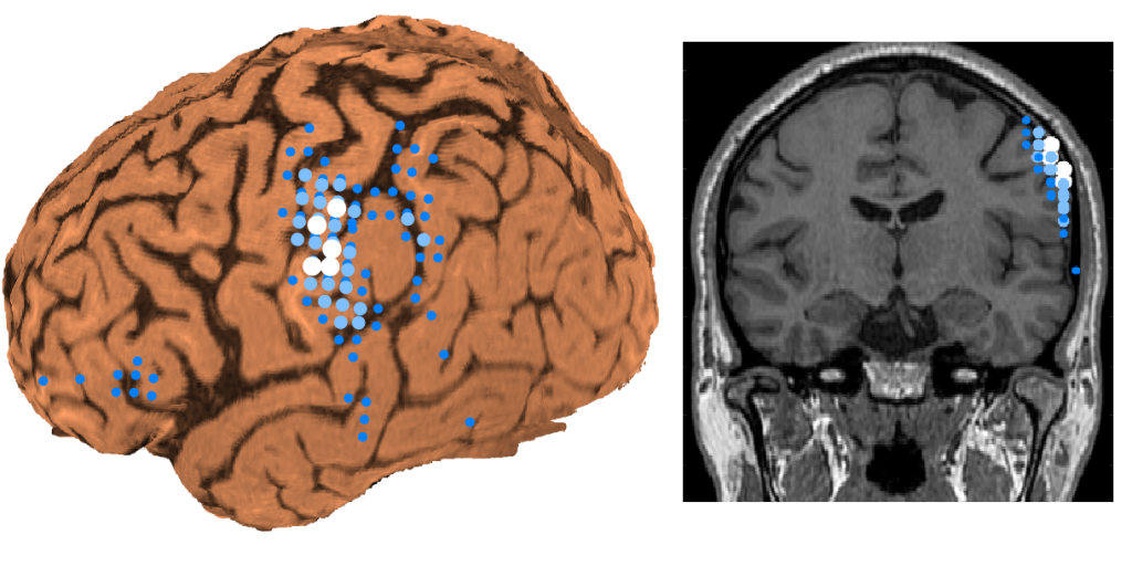
This is a basic solution for spatial filtering, and is called the Minimum Norm Estimate (MNE) [1]. The drawback of MNE is that it always overestimates the current moment of the source close to the sensor, resulting in a solution of glowing brain surface (see the figure below).

Thus, MNE alone is not suitable for situations where the signal source is assumed to be located some distance below the brain surface, and actually it is rarely used in papers of magnetoencephalography.
Summary: The solution of the current moment of the whole-brain \(\boldsymbol{q}=\boldsymbol{q}_{all}\) to the measured magnetic field \(\boldsymbol{b}\) is an underdetermined system, and using the whole-brain LFM \(\boldsymbol{L}=\boldsymbol{L}_{all}\), it can be written as \(\boldsymbol{q}=\boldsymbol{L}^{T}(\boldsymbol{L}\boldsymbol{L}^{T})^{-1}\boldsymbol{b}\).
In the next page, we will compare the Equivalent Current Dipole (ECD) estimation, a representative overdetermined solution, with the MNE, a basic underdetermined solution, and review the derivation process of each to see under what circumstances it is justified to adopt them as a solution to the inverse problem. Taking a closer look at the MNE also gives us an insight into the motivation behind the development of spatial filters.
(Reference)
- MS Hämäläinen, RJ Ilmoniemi: Interpreting magnetic fields of the brain: minimum norm estimates. Med Biol Eng Comput. 1994 Jan;32(1):35-42.